Shell and tube heat exchanger tutorial

This tutorial builds on the step-by-step conjugate heat transfer (CHT) example, extending it to more complex geometries and meshes, although the precedure is essentially the same. The tutorial is based on one for the preCICE coupling framework and at the end we directly compare with the preCICE results. The complete example can be found in Hippo's examples directory.

Overview

This tutorial contains three regions:

Tube (inner) region: cold fluid region inside the tubes of the heat exchanger.
Shell (outer) region: hot fluid region on the outside of the tubes containing baffles to enhance heat transfer
Solid region: copper tubes between the inner and outer fluid regions.

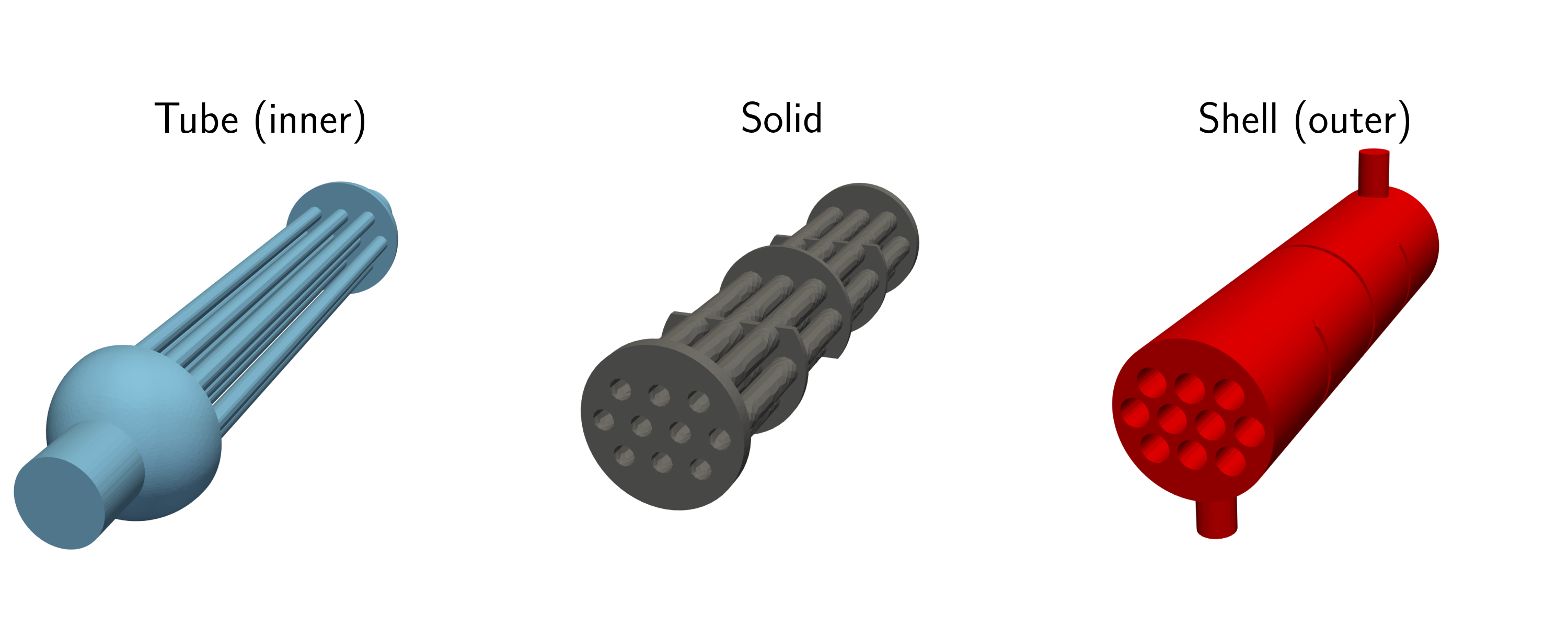
Solid and fluid domains of shell and tube heat exchanger

Coupling strategy

Hippo is currently capable of two CHT coupling strategies

Temperature-forward flux-back (TFFB): temperature imposed on solid, heat flux imposed on fluid. This was used in the step-by step example.
Flux-forward temperature-back (FFTB): heat flux imposed on solid, temperature imposed on fluid.

FFTB is used in this example. The choice between TFFB and FFTB is usually determined by the material properties of the fluid and solid region, with FFTB typically better when the solid has much higher thermal conductivity than the fluid. The drawback with FFTB, is that if all flux boundary conditions are used on the solid, a transient solve must be used, which can dramatically increase wall clock time.

Directory layout

download_meshes.sh: Downloads OpenFOAM meshes from the preCICE tutorial
solid.exo: mesh for the solid region in the Exodus II file format
fluid-inner-openfoam: OpenFOAM case directory for the tube region
fluid-outer-openfoam: OpenFOAM case directory for the shell region
solid.i: MOOSE input file for the solid region subject to heat conduction.
inner.i: Hippo input file for the tube region.
outer.i: Hippo input file for the shell region.
clean.sh: cleans case directories.
post.py: python script for postprocessing the results

Heat conduction problem

The solid region closely resembles that from the previous example, although in this case, the BCs are defined entirely by heat transfer from the fluid domain. Below we highlight some keys features of the solid solve that differ from the step-by-step example

Mesh

The solid mesh in this case has been generated for you and is a copy of the mesh used in the preCICE tutorial although converted into the Exodus II file format which is the most common format used by MOOSE. This is specified with


[Mesh]
    type = FileMesh
    file = 'solid.exo'
[]

Variables and kernels

A suble difference is the use of MOOSE's auto-differentiation kernels, with the AD prefix. This permits the automatic calculation of the Jacobian, allowing the Newton-Krylov solver to be used for more complex kernels (NEWTON is set in the Executioner block rather than PJFNK). For more information about the AD system see MOOSE's documentation.


[Variables]
    [T]
        family = LAGRANGE
        order = FIRST
        initial_condition = 300
    []
[]

[Kernels]
    [heat-conduction]
        type = ADHeatConduction
        variable = T
    []
    [heat-conduction-dt]
        type = ADHeatConductionTimeDerivative
        variable = T
    []
[]

Materials

The material propertes are set to those of copper, noting that the specific heat capacity, $var element = document.getElementById("moose-equation-5f4a68e0-351c-4b45-9f1e-217d1035bc92");katex.render("c_p", element, {displayMode:false,throwOnError:false});$ is initially reduced by a factor of 1000 to speed up the temperature development in the solid.


[Functions]
    [cp_func]
        type=ParsedFunction
        expression = 'if(t<50, 0.385, 385)'
    []
[]
[Materials]
    # Solid material properties for copper
    [thermal-conduction]
        type = ADGenericConstantMaterial
        prop_names = 'thermal_conductivity density'
        prop_values = '401 8960'  # W/(m.K) kg/m^3
    []
    [specific-heat]
        type=ADGenericFunctionMaterial
        prop_names = 'specific_heat'
        prop_values = cp_func
    []
[]

Fluid-Solid Coupling

Coupling is similar to the step-by-step example except there are two fluid domains and the FFTB scheme is being used. The MultiApps block looks like


[MultiApps]
    [inner]
        type = TransientMultiApp
        app_type = hippoApp
        execute_on = timestep_end
        input_files = 'inner.i'
        sub_cycling = true
    []
    [outer]
        type = TransientMultiApp
        app_type = hippoApp
        execute_on = timestep_end
        input_files = 'outer.i'
        sub_cycling = true
    []
[]

Imposing the solid temperature on OpenFOAM

The primary difference with the step-by-step example is that we now impose the temperature rather than heat flux on the fluid.

The data being transferred from MOOSE to OpenFOAM needs to consider the differences between finite element and finite volume methods. In the former, the temperature is defined continuously across element faces, whereas for the latter they are uniform.

This conversion is performed using a ProjectionAux on the inner and outer solid:


[AuxVariables]
    ...
    [wall_temp]
        family = MONOMIAL
        order = CONSTANT
        initial_condition = 300
    []
[]

[AuxKernels]
    [wall_temp]
        type = ProjectionAux
        variable = wall_temp
        v = T
        boundary = 'inner outer'
        check_boundary_restricted = false
    []
[]

Note that we have restricted the ProjectionAux to only apply to boundaries as in this case, we only need to consider data transfer there.

The Transfers block is used to define how the variables are transferred to the Hippo apps. In this case, we have used a nearest location transfer, which is often used on complex geometries, other options include using geometric interpolation.


[Transfers]
    [wall_temperature_to_outer]
        type = MultiAppGeneralFieldNearestLocationTransfer
        source_variable = wall_temp
        to_multi_app = outer
        variable = solid_wall_temp
        execute_on = same_as_multiapp
        from_boundaries = 'outer'
    []

    [wall_temperature_to_inner]
        type = MultiAppGeneralFieldNearestLocationTransfer
        source_variable = wall_temp
        to_multi_app = inner
        variable = solid_wall_temp
        execute_on = same_as_multiapp
        from_boundaries = 'inner'
    []
    ...
[]

The from_boundaries parameter is used here to restrict the nearest location search to the specified boundary.

In the Hippo input files, we use a FoamBCs block to impose the boundary conditions on the OpenFOAM domains. Both inner.i and outer.i are the same:


[FoamBCs]
    [solid_wall_temp]
        type = FoamFixedValueBC
        foam_variable = T
        initial_condition = 300
    []
[]

Note that this is a different type to the step-by-step example where a FoamFixedGradientBC is used.

Imposing the fluid heat flux on the solid

First, the heat flux must be computed for the OpenFOAM simulations. For both inner.i and outer.i, a FoamFunctionObject is used in the FoamVariables block:


[FoamVariables]
    [fluid_heat_flux]
        type = FoamFunctionObject
        foam_variable = wallHeatFlux
    []
[]

As the type suggests, this executes the wallHeatFlux OpenFOAM function object and shadows its output with a MOOSE variable called fluid_heat_flux which can be transferred to the solid app. solid.i needs AuxVariables to contain the variables sent from the inner and outer Hippo simulations.


[AuxVariables]
    [inner_heat_flux]
        family = MONOMIAL
        order = CONSTANT
        initial_condition = 0
    []
    [outer_heat_flux]
        family = MONOMIAL
        order = CONSTANT
        initial_condition = 0
    []
    ...
[]

solid.i must also transfer the heat flux from the inner and outer OpenFOAM simulations into the AuxVariables.


[Transfers]
    ...
    [heat_flux_from_inner]
        type = MultiAppGeneralFieldNearestLocationTransfer
        source_variable = fluid_heat_flux
        from_multi_app = inner
        variable = inner_heat_flux
        execute_on = same_as_multiapp
        to_boundaries = 'inner'
    []
    [heat_flux_from_outer]
        type = MultiAppGeneralFieldNearestLocationTransfer
        source_variable = fluid_heat_flux
        from_multi_app = outer
        variable = outer_heat_flux
        execute_on = same_as_multiapp
        to_boundaries = 'outer'
        search_value_conflicts=false
    []
[]

The AuxVariables must then be imposed as boundary conditions using coupledVarNeumannBC type


[BCs]
    [inner]
        type = CoupledVarNeumannBC
        variable = T
        boundary = inner
        v = inner_heat_flux
        scale_factor=-1
    []

    [outer]
        type = CoupledVarNeumannBC
        variable = T
        boundary = outer
        v = outer_heat_flux
        scale_factor=-1
    []
[]

The -1 scale factor is used as the FoamFunctionObject gives the outward normal wall heat flux. The CoupledVarNeumannBC is also defined using the outward normal to the MOOSE boundary so the sign must be reversed to account for heat travelling from the fluid to the solid.

Running and visualising the case

The case, including downloading and partitioning the meshes, can be run using ./run.sh.

Visualisation using `pyvista`

pyvista is pythonic VTK (Visualisation Toolkit) wrapper that allows high quality 3D data to be plotted. This can be installed using


pip install pyvista

Use python post.py to display the heat exchanger.

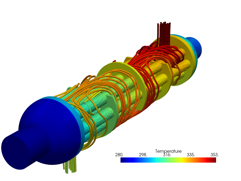
Hippo results showing streamlines in the outer region

The results can also be compared with the preCICE tutorial as the same meshes have been used. For the fluid domains the relative errors are shown below

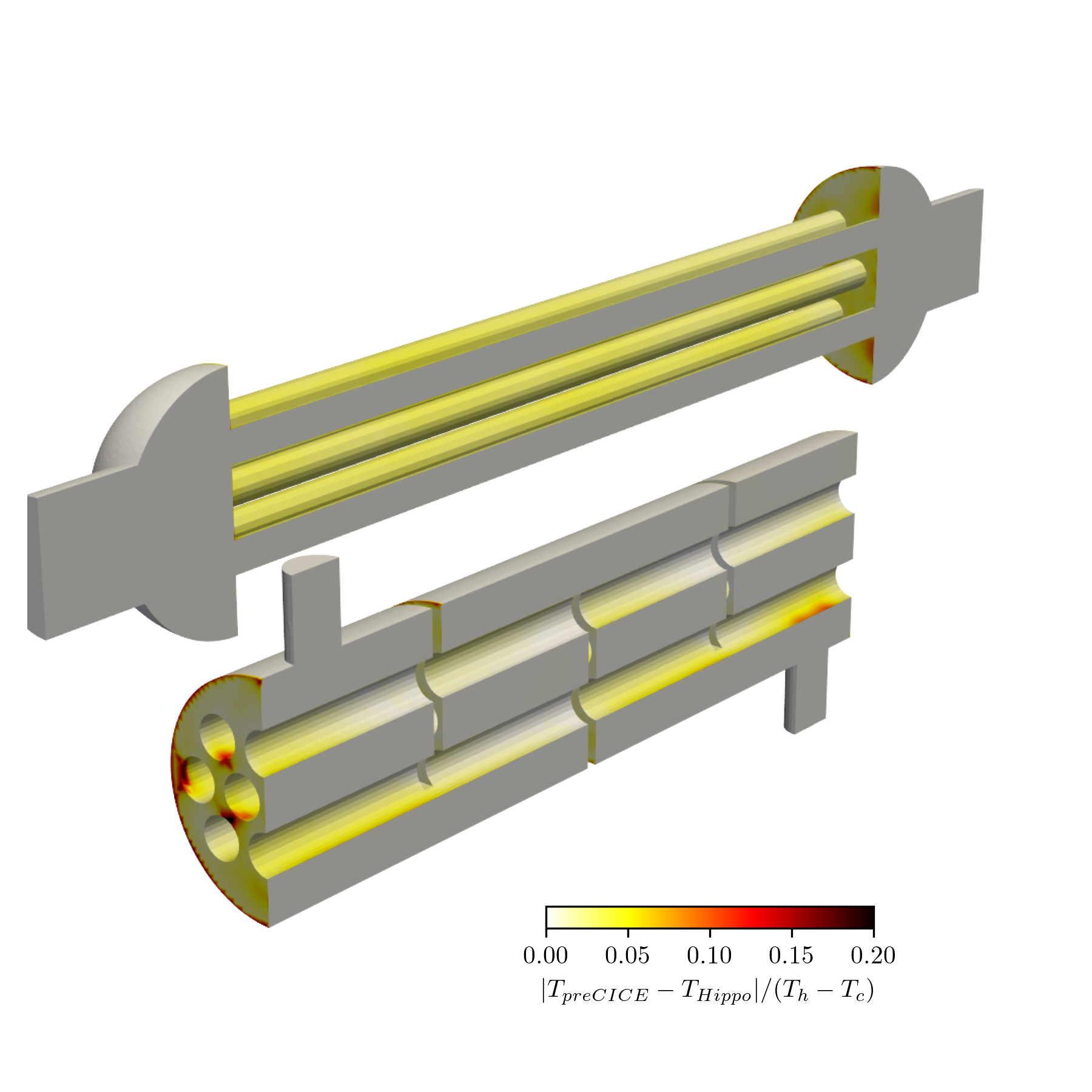
Pointwise comparison with preCICE tutorial.

The differences are small except close to the boundaries and particularly in the corners, this is likely due to the different coupling strategies,

Overview
Directory layout
Heat conduction problem
Fluid - Solid Coupling
Imposing the fluid heat flux on the solid
Running and visualising the case